The Reports page allows you to run Monte Carlo reports of the tasks in the project, such as: Cumulative Curves, Tornado, Status and Previews. The reports are run based on the scenario applied for the project.
Monte Carlo Charts:
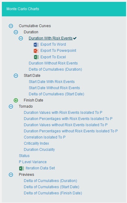
Figure 1
2.10.1 Cumulative Curves:
The Cumulative Curves report includes Duration: Duration with Risk Events, Duration without Risk Events, Delta of Cumulatives (Duration); Start Date: Start Date with Risk Events, Start Date without Risk Events, Delta of Cumulatives (Start Date); Finish Date: Finish Date with Risk Events, Finish Date without Risk Events, Delta of Cumulatives (Finish Date). The Cumulative Curve report shows the distribution of the estimated duration exposure of a selected project or task. It simulates duration values based on distribution types. The columns show the hits for each of the total amount of task simulation duration exposure.
The steps that are carried out to generate Cumulative Curves chart are as follows:
Step 1: Generate risk groups for the given correlations. Grouping is done such that all the tasks that are correlated with one another are considered as a group.
Step 2: Generate correlated random values for each risk group. The static calculation is explained below:
a) Create a correlation matrix with correlation coefficients such that task which is more correlated comes in the first row.
A correlation matrix is used to investigate the dependence between multiple variables at the same time. The result is a table containing the correlation coefficients between each variable and the others.
b) Calculate unspecified coefficients in the matrix from correlation of two related specified correlation coefficients.
b.1: Find Eigen values and Eigen vectors matrices of the inconsistent correlation matrix.
b.2: Replace the non-positive Eigen values with the smallest positive double number.
b.3: Create a Diagonal Matrix of Sqrt (1 / (Eigen Vectors^2 * Eigen Values))
b.4: Create a Diagonal Matrix of Sqrt (Eigen Values)
b.5: Multiply the diagonal matrix in step 3 with Eigen vectors matrix which is multiplied the matrix in step 4.
i.e., Diagonal Matrix of Sqrt (1 / (Eigen Vector^2 * Eigen Values)) * Eigen Vector * Diagonal Matrix of Sqrt (Eigen Values)
b.6: Multiply the matrix got from step 5 with its transpose. Now we will get the correlation matrix which is consistent.
b.7: Replacing the inconsistent coefficients with coefficients calculated from consistent coefficients. ? = (6 * asin(Correlation Coefficient / 2) /p) * 100
c) Perform cholesky decomposition of the correlation matrix (CHOL). If exception occurs, then the correlation matrix is inconsistent. Then the simulation is stopped and asks the user whether to adjust correlations of the risk group automatically or not. If no exception occurs, then perform the remaining steps.
The Cholesky decomposition or Cholesky factorization is a decomposition of a Hermitian, positive-definite matrix into the product of a lower triangular matrix and its conjugate transpose, which is useful example for efficient numerical solutions and Monte Carlo simulations.
d) Create a matrix (R) with number of rows is equal to iteration times and number of columns equal to number of tasks in the risk group with randomly generated values which are normally distributed with mean 0 and SD 1.
e) Multiply the matrix generated in (d) with matrix generated by cholesky decomposition. This gives the normally distributed random values with correlation (these values used in normally distributed duration). To get it uniformly distributed, find the cumulative distribution function of the matrix (these values are used for other distributions). Each columns will have the random values for corresponding task duration.
I.e., correlated random value matrix CRM is
CRM = R * CHOL, if normal distribution
CRM = pnorm(R * CHOL), if not normal distribution
The cumulative distribution function (CDF) of a real-valued random variable X, or just distribution function of X, evaluated at x, the probability that X will take a value less than or equal to x.
Example
An example for normal distribution with 10 iterations is given below.
a) Let A, B, C, D are correlated such that corr (A, B) = 60%, corr (A, C) = 70%, corr (A, D) = 80%. Now we have one risk group ABCD.
b) Correlation Matrix with user specified correlation coefficients
| 1.0 | 0.6 | 0.7 | 0.8 |
| 0.6 | 1.0 | 0.0 | 0.0 |
| 0.7 | 0.0 | 1.0 | 0.0 |
| 0.8 | 0.0 | 0.0 | 1.0 |
Table 1
c) Correlation Matrix after calculating all correlation coefficients
| 1.0 | 0.5112 | 0.5936 | 0.6748 |
| 0.5112 | 1.0 | 0.0302 | 0.0343 |
| 0.5936 | 0.0302 | 1.0 | 0.0398 |
| 0.6748 | 0.0343 | 0.0398 | 1.0 |
Table 2
d) Matrix with random values, R
| -0.22759883330513203 | -0.14779528819416274 | -0.8116534929634235 | -1.3828258408574279 |
| -0.6257058657442784 | 0.22979287727014666 | 0.6940068141614696 | -1.2819970948797965 |
| 0.9606080643281025 | 0.12951392609894774 | 0.9969510606030434 | 0.5490356353852022 |
| -1.0168529345485386 | -0.7515175581895532 | 0.33692856764956125 | -1.3325301102147291 |
| -0.672674228450859 | 0.8940508933639131 | -1.5357821937125395 | -0.38541097828943366 |
| 0.8837124607600431 | 0.21956223049086745 | 0.4804300141584299 | 0.8033496303121265 |
| -2.080382126627115 | -1.4204197286554967 | -0.8921771773333548 | -1.4384490197892787 |
| -0.9457988314984864 | -0.16309395713329183 | -0.30523272399453705 | -1.0969624106348446 |
| -0.6255515357453936 | 1.2239957073107248 | -0.36742658070420897 | -1.5732911013915596 |
| -0.0612578037946805 | -0.34877000727229757 | -1.1554191662901698 | 1.1669823548362461 |
Table 3
e) Matrix with correlated random values
| Task A | Task B | Task C | Task D |
| -0.22759883330513203 | -0.14779528819416274 | -0.8116534929634235 | -1.3828258408574279 |
| -0.6257058657442784 | 0.22979287727014666 | 0.6940068141614696 | -1.2819970948797965 |
| 0.9606080643281025 | 0.12951392609894774 | 0.9969510606030434 | 0.5490356353852022 |
| -1.0168529345485386 | -0.7515175581895532 | 0.33692856764956125 | -1.3325301102147291 |
| -0.672674228450859 | 0.8940508933639131 | -1.5357821937125395 | -0.38541097828943366 |
| 0.8837124607600431 | 0.21956223049086745 | 0.4804300141584299 | 0.8033496303121265 |
| -2.080382126627115 | -1.4204197286554967 | -0.8921771773333548 | -1.4384490197892787 |
| -0.9457988314984864 | -0.16309395713329183 | -0.30523272399453705 | -1.0969624106348446 |
| -0.6255515357453936 | 1.2239957073107248 | -0.36742658070420897 | -1.5732911013915596 |
| -0.0612578037946805 | -0.34877000727229757 | -1.1554191662901698 | 1.1669823548362461 |
Table 4
Each column in the matrix contains the random values for corresponding tasks for each iteration.
Step 3: Generate random values for resources of those tasks which are not correlated.
Step 4: Generate random values for resource rates of those tasks which are not correlated.
Step 5: Set the random values of resources as random values for resource rates of those tasks which are correlated.
Step 6: For each resource of a task generate values based on the distribution and number of iterations with given uncertainties. For import type “Multiple Resources”, there can be multiple resources for a task and the uncertainties may be different for each of them.
Step 7: Generate values based on the distribution and number of iterations with given uncertainties for corresponding resource rate of each resource. For import type “Simple Uncertainty”, the values will be same for all iteration.
Step 8: For each iteration, multiply the values of resource and resource rate respectively to find the duration for each resource.
Step 9: For each iteration, add the duration of all resources.
2.10.1.1 Duration with Risk Events:
The Duration report shows the distribution of the estimated duration exposure of a selected project or task. It simulates duration values based on distribution types. The columns show the hits for each of the total amount of task simulation duration exposure. The curve shows the cumulative frequency of the hits in percentage. To get individual task´s Cumulative Curve report, select the task from the PROJECT REPORT dropdown.
Steps:
- Simulations —>Reports
- Click Duration with Risk Events link under Cumulative Curves. (Figure 1)
- Select the Bar width and set the Iteration Times and then click RUN ANALYSIS (Figure 2) The chart generated and the table is shown in the Figure 2.
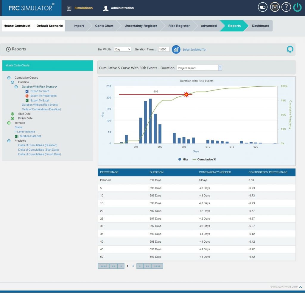
Figure 2
2.10.1.2 Duration without Risks Events:
The Duration report shows the distribution of the estimated duration exposure of a selected project or task without considering the risks associated with it. It simulates duration values based on distribution types. The columns show the hits for each of the total amount of task simulation duration exposure. The curve shows the cumulative frequency of the hits in percentage.
Steps:
- Simulations—>Reports
- Click Duration without Risk Events link under Cumulative Curves. (Figure 1)
- Select the Bar width and set the Iteration Times and then click RUN ANALYSIS (Figure 3) The chart generated and the table is shown in the Figure 3
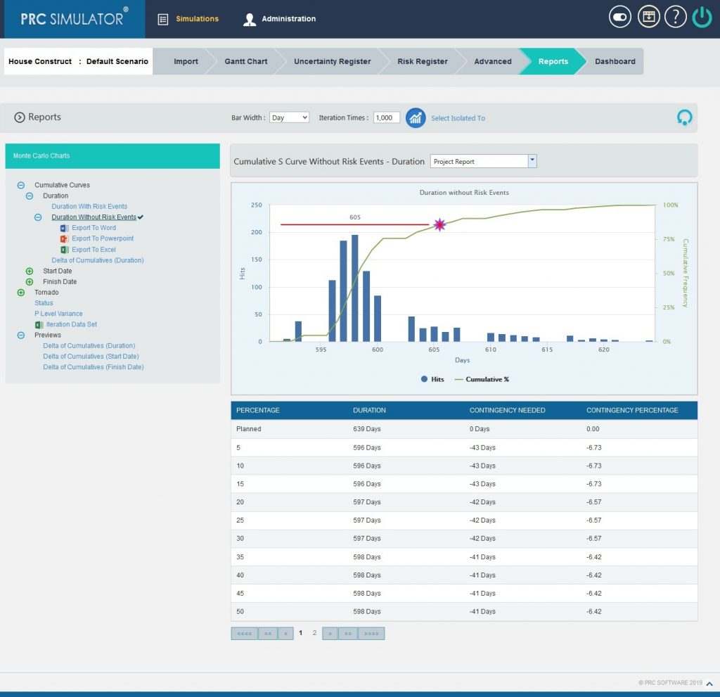
Figure 3
2.10.1.3 Delta of Cumulatives (Duration):
The Delta of Cumulative chart shows the variation Curve of durations with risk and without risk.
This chart appears after running the simulation for the first time.
Steps:
- Simulations—>Reports
- Click Delta of Cumulatives(Duration) link under Cumulative Curves. (Figure 1)
- Set the Iteration Times and then click RUN ANALYSIS (Figure 4) The chart generated and the table is shown in the Figure 4.
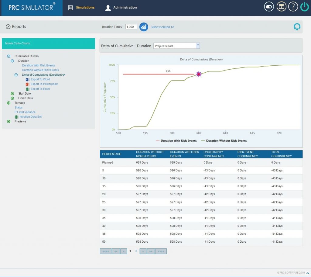
Figure 4
2.10.1.4 Start Date with Risk Events:
Steps:
- Simulations —>Reports
- Click Start Date with Risk Events link under Cumulative Curves. (Figure 1)
- Select the Bar width and set the Iteration Times and then click RUN ANALYSIS (Figure 5) The chart generated and the table is shown in the Figure 5.

Figure 5
2.10.1.5 Start Date without Risk Events:
Steps:
- Simulations—>Reports
- Click Start Date without Risk Events link under Cumulative Curves. (Figure 1)
- Select the Bar width and set the Iteration Times and then click RUN ANALYSIS (Figure 6) The chart generated and the table is shown in the Figure 6
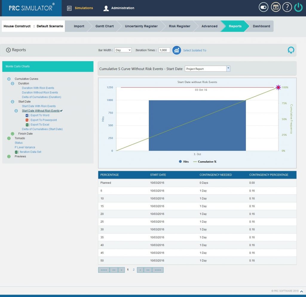
Figure 6
2.10.1.6 Delta of Cumulatives (Start Date):
The Delta of Cumulative chart shows the variation Curve of start date with risk and without risk.
This chart appears after running the simulation for the first time.
Steps:
- Simulations—>Reports
- Click Delta of Cumulatives (Start Date) link under Cumulative Curves. (Figure 1)
- Set the Iteration Times and then click RUN ANALYSIS (Figure 7) The chart generated and the table is shown in the Figure 7.
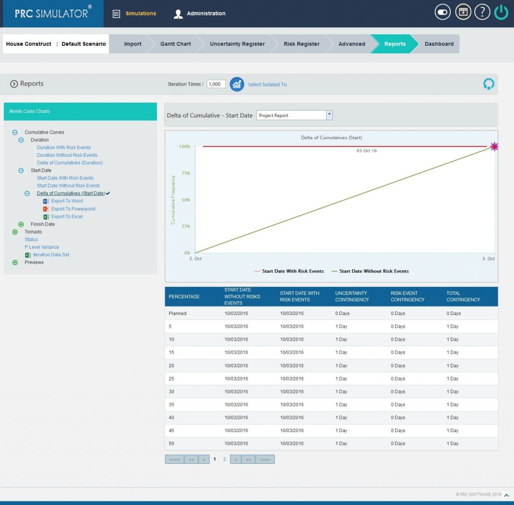
Figure 7
2.10.1.7 Finish Date with Risk Events:
Steps:
- Simulations —>Reports
- Click Finish Date with Risk Events link under Cumulative Curves. (Figure 1)
- Select the Bar width and set the Iteration Times and then click RUN ANALYSIS (Figure 8) The chart generated and the table is shown in the Figure 8.
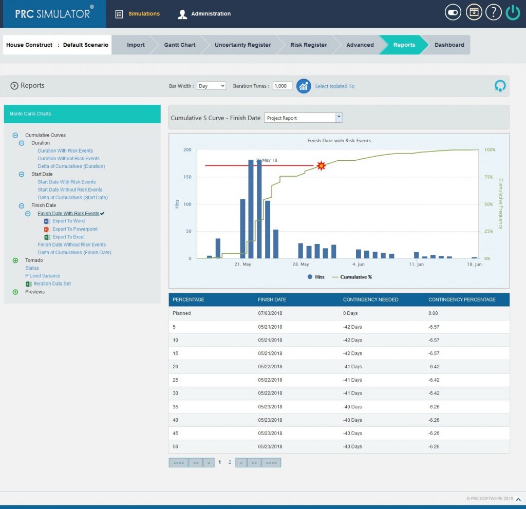
Figure 8
2.10.1.8 Finish Date without Risk Events:
Steps:
- Simulations—>Reports
- Click Finish Date without Risk Events link under Cumulative Curves. (Figure 1)
- Select the Bar width and set the Iteration Times and then click RUN ANALYSIS (Figure 9) The chart generated and the table is shown in the Figure 9
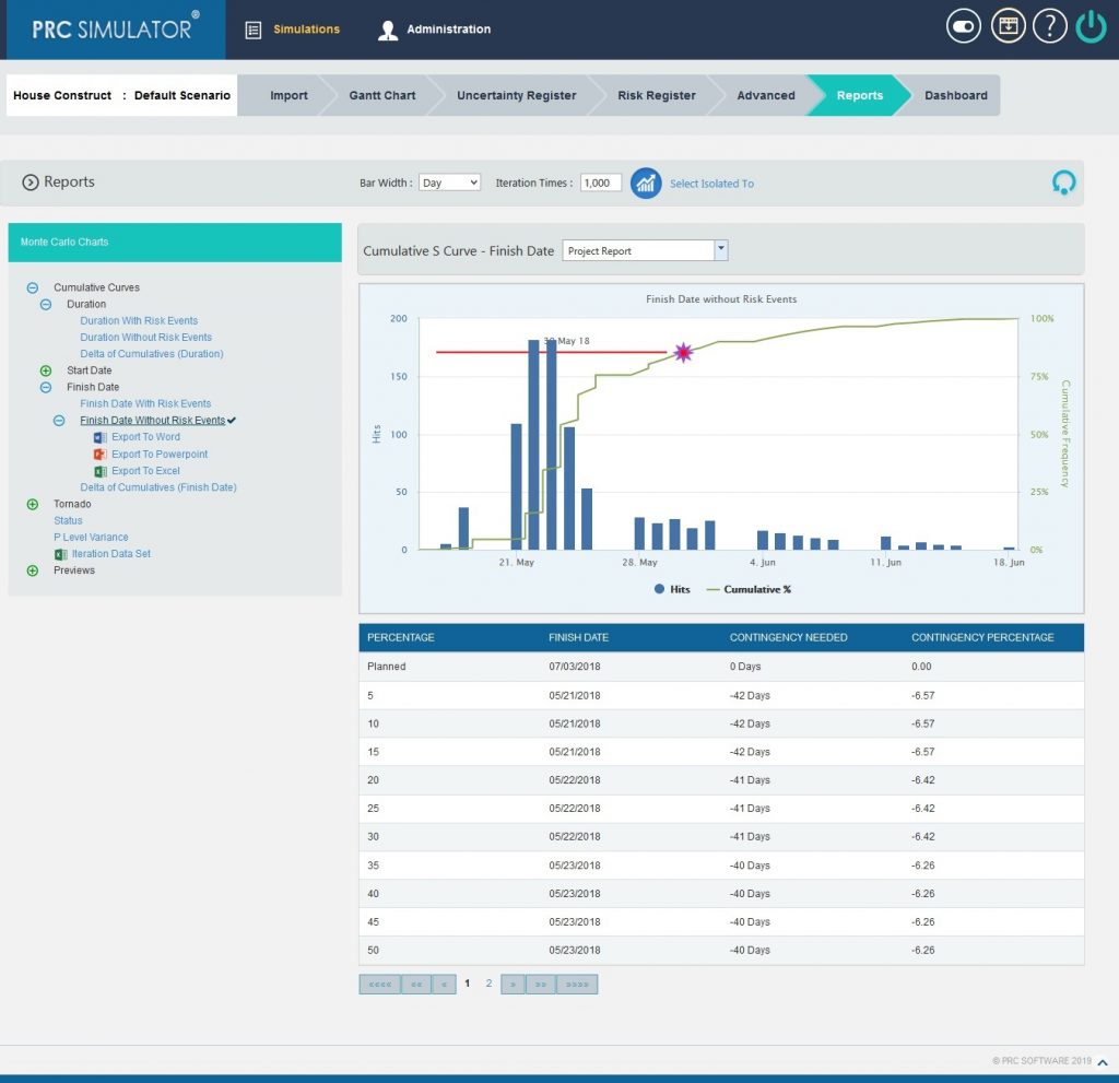
Figure 9
2.10.1.9 Delta of Cumulatives (Finish Date):
The Delta of Cumulative chart shows the variation Curve of finish date with risk and without risk.
This chart appears after running the simulation for the first time.
Steps:
- Simulations—>Reports
- Click Delta of Cumulatives (Finish Date) link under Cumulative Curves. (Figure 1)
- Set the Iteration Times and then click RUN ANALYSIS (Figure 10) The chart generated and the table is shown in the Figure 10.
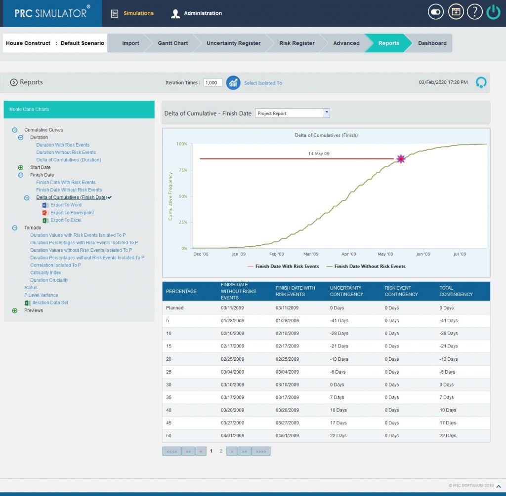
Figure 10
2.10.2 Tornado Charts:
The Duration Values with Risk Events Isolated To P, Duration Percentages with Risk Events Isolated To P, Duration Values without Risk Events Isolated To P, Duration Percentages without Risk Events Isolated To P, Correlation Isolated to P, Criticality Index and Duration Cruciality reports are Tornado Charts that depends on the simulated duration exposure values of each task up to the Pn iteration value, where `n´ is the percentile value of total number of iterations given. The x axis represents the duration exposure and the y axis represents the task names.
2.10.2.1 Duration Values with Risk Events Isolated To P:
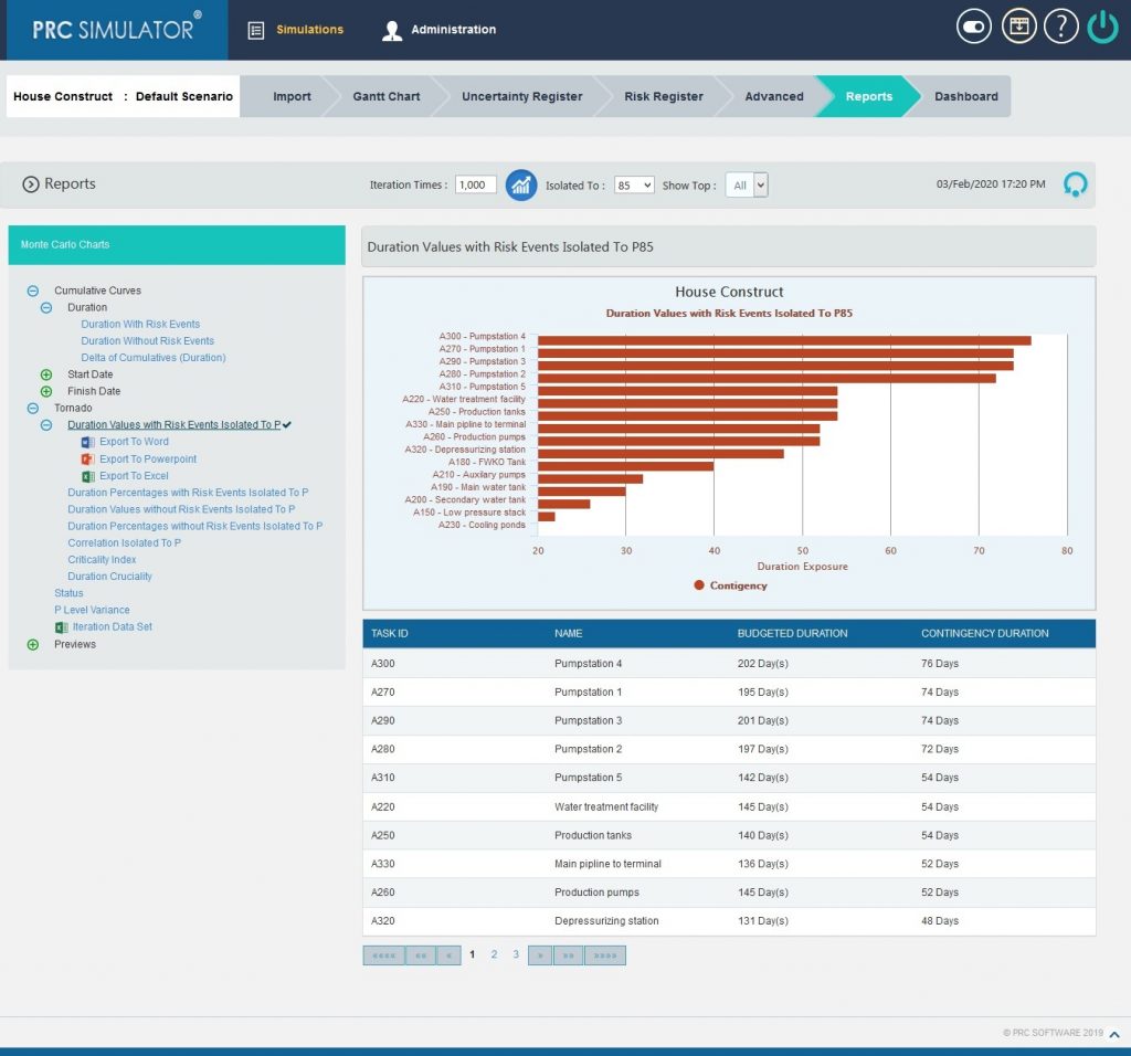
Figure 11
2.10.2.2 Duration Percentages with Risk Events Isolated To P:

Figure 12
2.10.2.3 Duration Values without Risk Events Isolated To P:
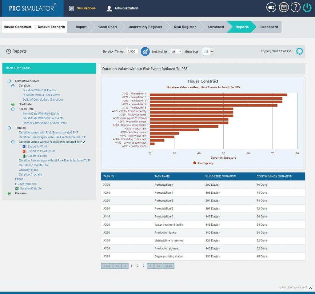
Figure 13
2.10.2.4 Duration Percentages without Risk Events Isolated To P:
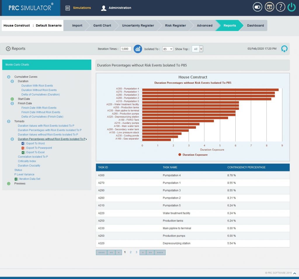
Figure 14
2.10.2.5 Correlation Isolated to P:
The step to generate the Correlation Isolated to P (n) chart is:
Pearson correlation coefficient for Total duration up to p(n) and Task duration up to p(n) * 100
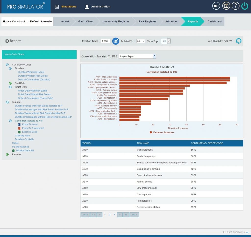
Figure 15
2.10.2.6 Criticality Index:
The tasks which are highly critical to be completed for the project are shown in the top followed by all other tasks.
The arrow button in the right side of the chart as in the Figure 16 allows navigating UP or DOWN through all the tasks associated with the project.
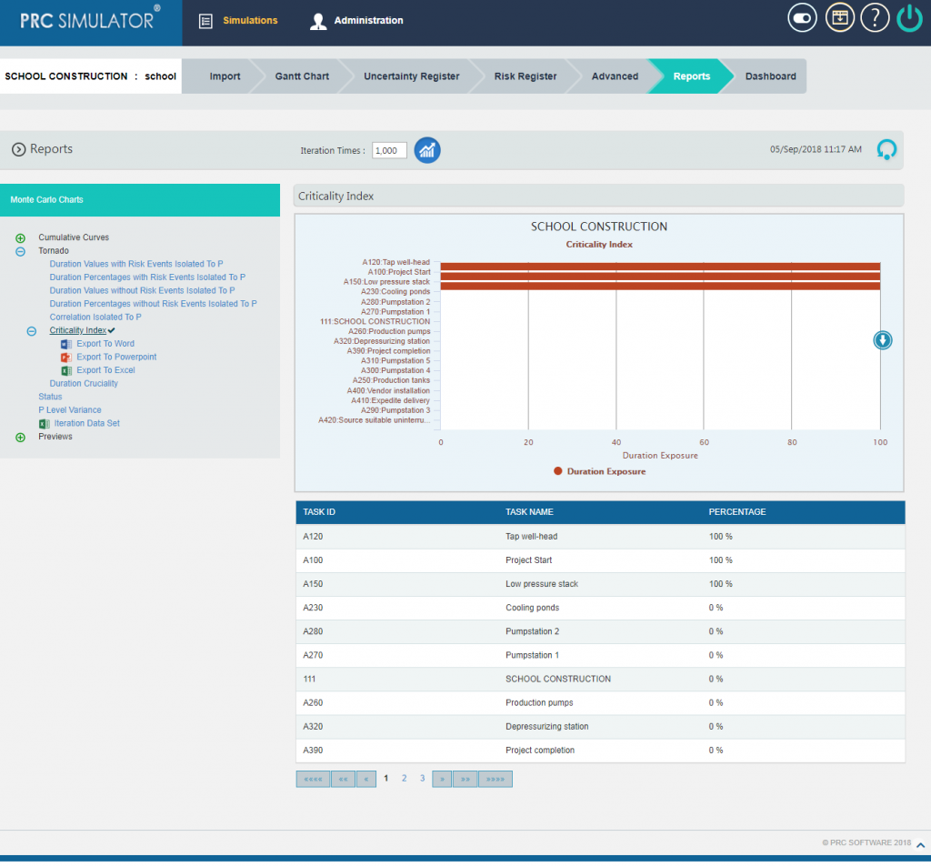
Figure 16
2.10.2.7 Duration Cruciality
The tasks which are crucial for the successful completion of the project are shown in the top followed by all other tasks.
The arrow button in the right side of the chart as in the Figure 17 allows navigating UP or DOWN through all the tasks associated with the project.
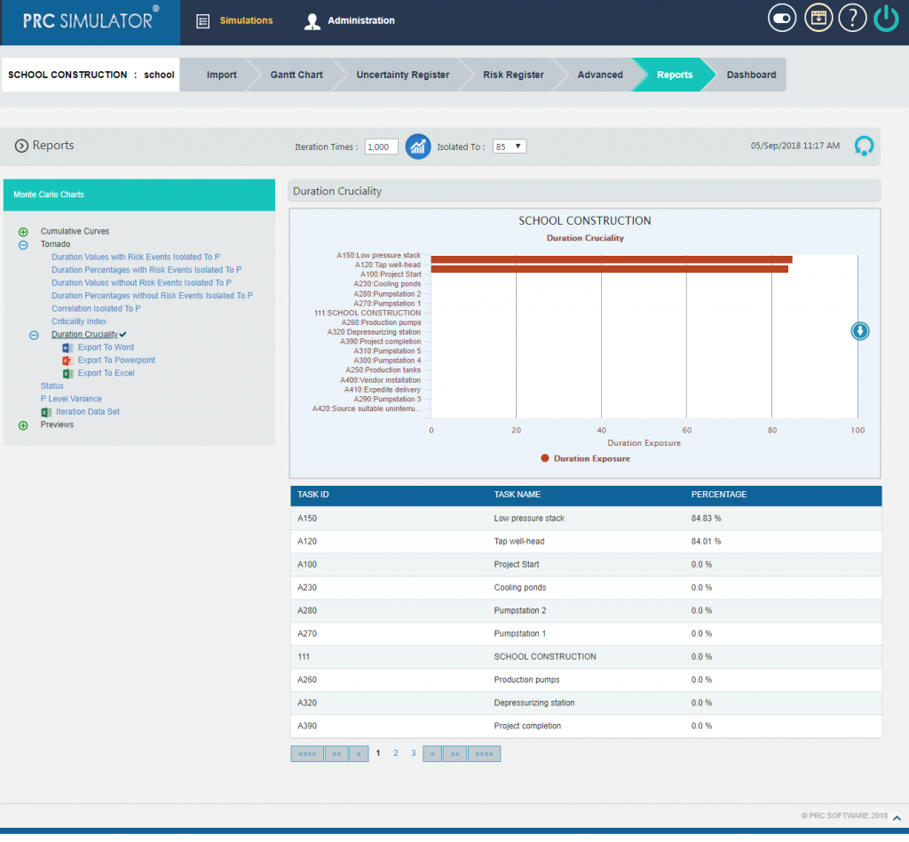
Figure 17
2.10.2.8 Status charts:
This Monte Carlo chart is a pie chart which shows the total number of tasks included in the project. And the number of risks mapped to the tasks as threat and opportunities are also counted.
Steps:
- Simulations —> Reports
- Click Status link under Monte Carlo Charts. (Figure 1) The chart generated and the table is shown in the Figure 18.
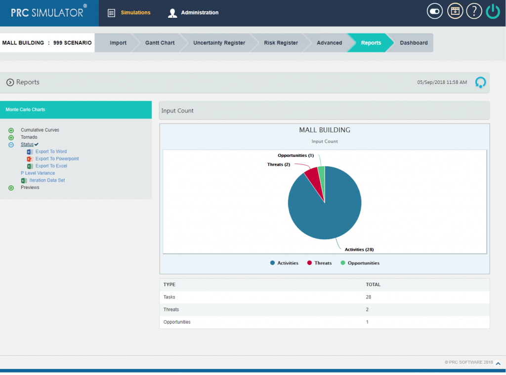
Figure 18
2.10.3 P Level Variance
It is an Area Range Chart that plots the difference between Upper P value and Lower P Value for all Tasks in the selected Project or individual Tasks for the selected Upper P value and Lower P value.
Steps:
- Simulations —> Reports
- Click P Level Variance link under Monte Carlo Charts. (Figure 1)
- Set the Iteration Times and after selecting the lower and upper bounds, Click OK button then click RUN ANALYSIS icon. The chart generated is on the basis of Variance between Upper and Lower P value by default and the table as shown in the Figure 19.
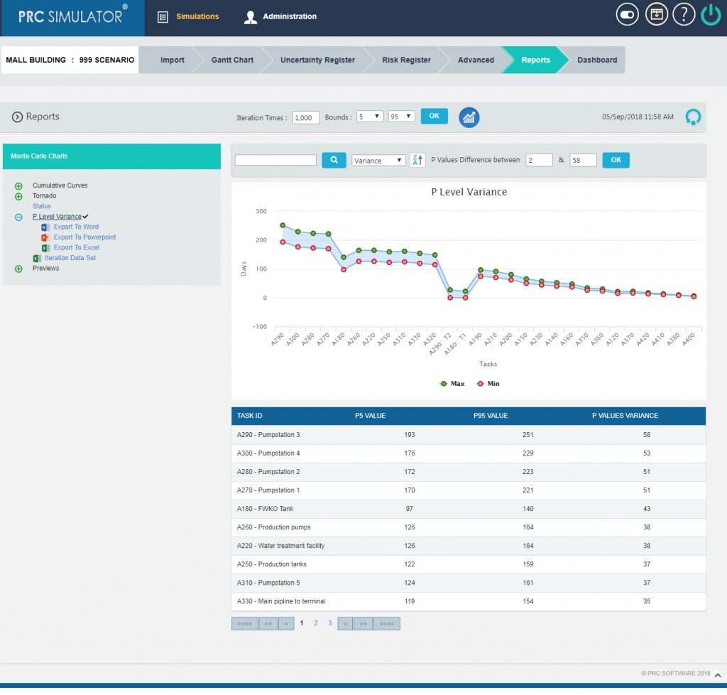
Figure 19
The chart can also be generated on the basis of Upper Bound values (Figure 20) , Lower Bound values (Figure 21) and Task IDs (Figure 22) by selecting the same from the drop down.

Figure 20
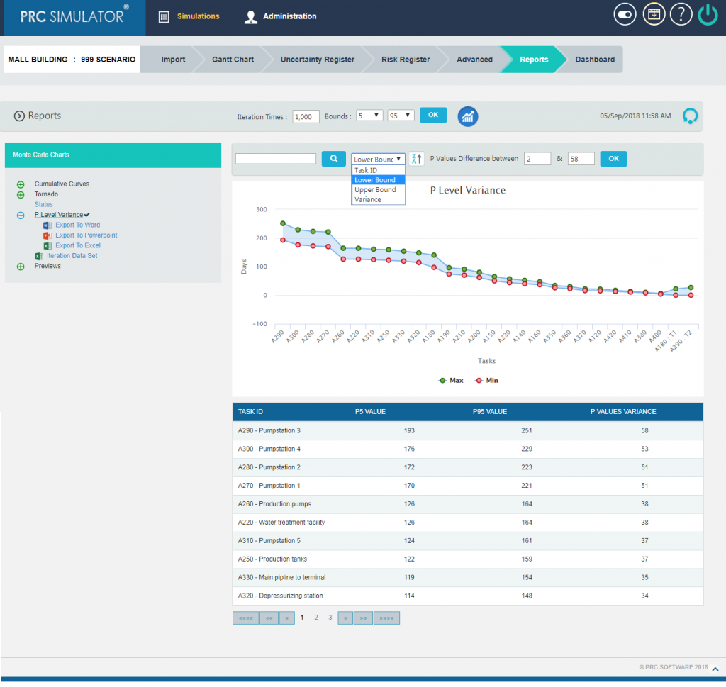
Figure 21
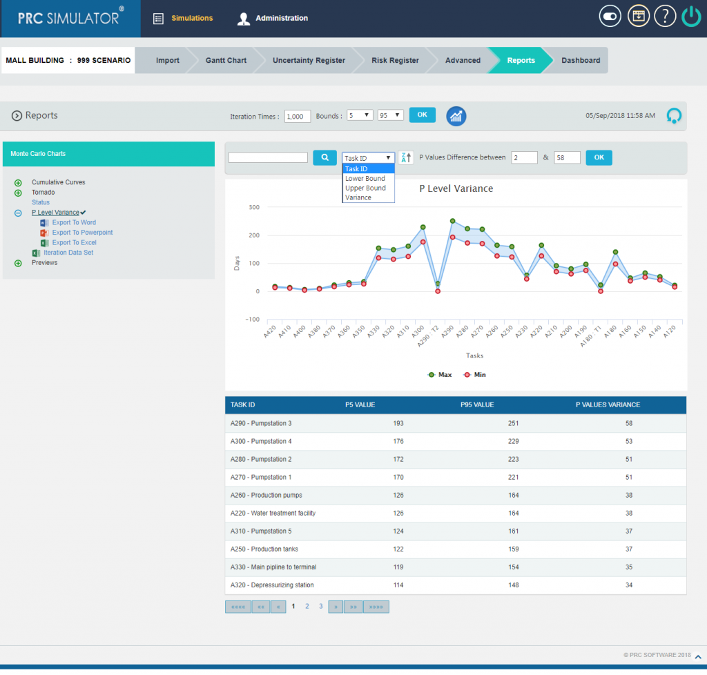
Figure 22
The chart is provided with sort option, which sorts the graph and table for the given criteria as in Figure 23.
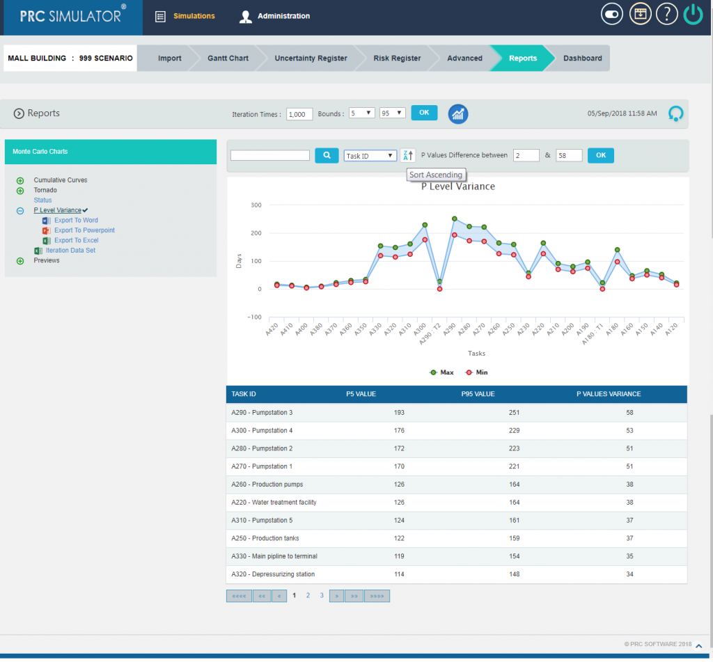
Figure 23
Also there are ways to filter the Tasks for P Level Variance Chart on the basis of the variance between the P Values and Task ID as in Figure 24.
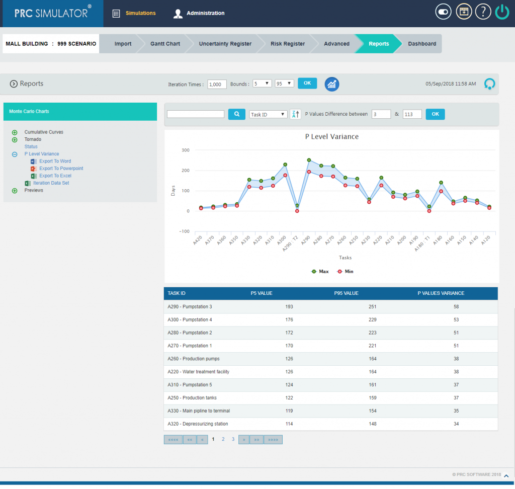
Figure 24
2.10.3.1 Iteration Data Set:
This functionality is used to export the tasks with risk events and without risk events along with Task Id, Task Name and Planned Duration of the selected project to MS Excel. A sample spreadsheet is shown in Figure 25. Iterations value are calculated for each task separately based on the number of iteration specified.
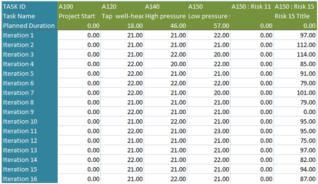
Figure 25
2.10.4 Previews:
The Preview Charts are used to get the previews of Delta of Cumulative Curves with approximate values before running the simulation. It shows two S-Curves. The first S-Curve shows the cumulative frequency of the item with risks, and the other shows Cumulative Frequency of the item without risks. Thus the two curves show the approximate result variation occurring when simulating with risk and without risk.
2.10.4.1 Delta of Cumulatives (Duration):
The Delta of Cumulative chart shows the variation Curve of duration with risk and without risk.(Figure 26)
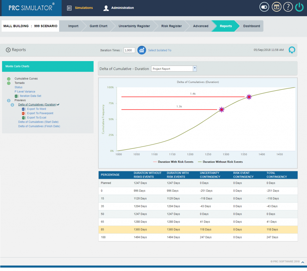
Figure 26
2.10.4.2 Delta of Cumulatives (Start Date):
The Delta of Cumulative chart shows the variation Curve of start date with risk and without risk.(Figure 27)
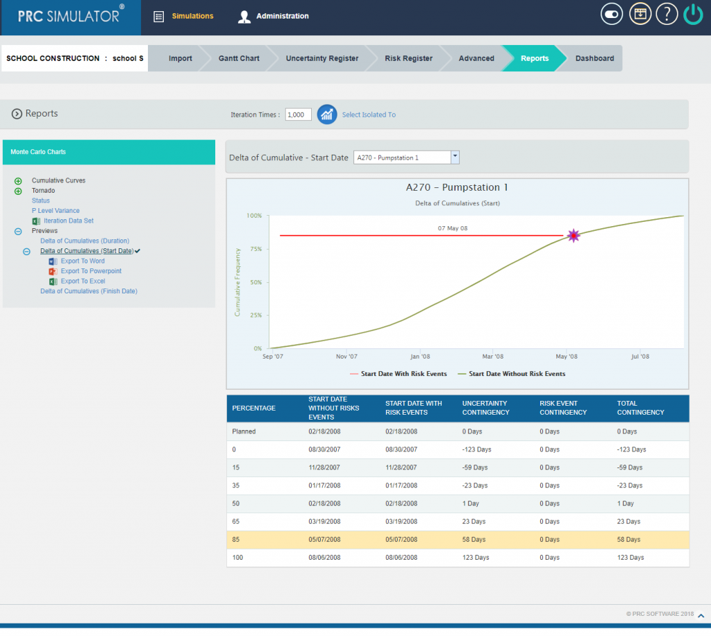
Figure 27
2.10.4.3 Delta of Cumulatives (Finish Date):
The Delta of Cumulative chart shows the variation Curve of finish date with risk and without risk.(Figure 28)
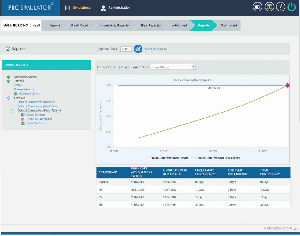
Figure 28
2.10.5 Export to Word:
This functionality is used to export the Simulation Monte Carlo reports and data table as a Word document.
Steps:
- Simulations —> Reports
- Click the Export to Word link. (Figure 1)
2.10.6 Export to PowerPoint:
This functionality is used to export the Simulation Monte Carlo reports generated to PowerPoint.
Steps:
- Simulations —> Reports
- Click the Export to PowerPoint link. (Figure 1)
2.10.7 Export to Excel:
This functionality is used to export the Simulation Monte Carlo reports as an excel file.
Steps:
- Simulations —> Reports
- Click the Export to Excel link. (Figure 1)